The Advection-Diffusion Equation models the distribution of a pollutant quantity in some medium (i.e. a fluid). It comprises two parts:
The diffusion term describes the dispersion of the concentration due to molecular motion, according to the diffusivity ;
The advection term represents the motion of the concentration due to being carried with the medium’s velocity field ;
The transient term relates the time evolution of to the other two spatial derivatives.
These two terms together describe the evolution in time of the concentration :
This lesson is about using pystencils to simulate a simple two-dimensional advection-diffusion scenario. We will discretize the ADE using a second-order finite difference scheme in space, and first-order explicit Euler integration in time; set up boundary conditions and an integration loop, and visualize the results. As an extra perk, we will build the entire solver to be accellerated by your machine’s graphics processor (GPU) [1].
During this lesson, you will use pystencils to construct a solver for a simple two-dimensional, time-dependent problem governed by the advection-diffusion equation. In the process, you will
derive an integration rule for the ADE using second-order finite differences in space, and an explicit Euler scheme in time;
implement a Neumann boundary condition as a pystencils operator;
implement a localized mass source using a guarded operator;
accelerate your simulation by running it on the GPU;
and use PyVista to interactively visualize your simulation results.
Let’s start by importing the packages we will need.
import sympy as sp
import pystencils as ps
import numpy as np
import pyvista as pv

interactive_plots = FalseGPU Target Selection
Up to this point, we have only generated non-optimized kernel code for CPU execution. Pystencils, however, is built to harness the parallel processing power that is now built into most computers, from your laptop up to exascale computing clusters.
One major driver of that parallelism are general-purpose graphics processing units (GPUs). If you have a GPU, you can use it to accelerate your pystencils operators with only minimal changes to your code - without the need to get into the details of GPU kernel programming.
Notebook Cell
for t in ps.Target.available_targets():
    if t.is_gpu():
        target = t
        break
else:
    target = ps.Target.CurrentCPU
Create Algebraic Objects
Let’s begin building our ADE simulation by setting up algebraic objects for our simulation domain, variables, and fields.
Notebook Cell
L = (200, 80)
Ω = ps.grids.Patch("Ω", L, num_vertices=(lx + 1 for lx in L))

D, Δx, Δt = sp.symbols("D, Δx, Δt")

c = ps.grids.TensorField("c", Ω.vertices, ())
v = ps.grids.TensorField("v", Ω.vertices, (2,))
Implement the Integrator
Next up, we implement the time-integration operator for the advection-diffusion equation. To do so, we first need to take a look at our discretization scheme. We can discretize the three derivative terms separately, like follows:
For the diffusion term , we make the simplifying assumption that is constant across the domain. It thus simplifies to with the Laplace operator . To discretize, we apply the same second-order finite difference stencil as in the previous lesson to receive:
The advection term , signifies the divergence of the vector field :
To discretize, we simply apply central differences to the two spatial derivatives:
The transient term we discretize via a forward-Euler difference:
By rewriting (1), this gives rise to the following explicit update scheme:
Notebook Cell
c_next = ps.grids.TensorField("c_next", Ω.vertices, ())


@ps.flow.operator(
    target=target,
    ispace=Ω.vertices[1:-1, 1:-1]
)
def integrate_ade(_eq):
    _eq.let[Δx] = Ω.spacing[0]

    diff, advc = sp.symbols("diff, advc")
    _eq.let[diff] = D * (
                          c[-1, 0]()
                        + c[1, 0]()
                        + c[0, -1]()
                        + c[0, 1]()
                        - 4*c[0, 0]()
                    ) / Δx**2
    _eq.let[advc] = (
                        c[1, 0]()*v[1, 0](0) - c[-1, 0]()*v[-1, 0](0)
                        + c[0, 1]()*v[0, 1](1) - c[0, -1]()*v[0, -1](1)
                    ) / (2*Δx)

    transient = (c_next() - c()) / Δt
    euler_update = sp.solve(transient - diff + advc, c_next())[0]
    _eq.store[c_next()] = euler_update
Prepare the Simulation Scenario
Our next step is to set up the simulation data. This includes allocating the field arrays, as well as initializing the field to a velocity profile along which the quantity will be advected.
If we want to run our simulation on the GPU, the data arrays must accordingly be allocated in GPU
memory. The PatchData class takes care of this automatically if we tell it which target we are running on.
Notebook Cell
Ω_data = ps.grids.PatchData(
    Ω,
    {
        D: 1.7,
        Δt: 0.01
    },
    target=target,
    fields=[c, c_next, v]
)
Initialize the Velocity Field
Notebook Cell
@ps.flow.operator(target=target)
def set_v(_eq):
    y, t, r, v_max = sp.symbols("y, t, r, v_max")
    _eq.let[y] = Ω.vertex()[1]
    _eq.let[r] = Ω.extents[1] / 2
    _eq.let[t] = 1 - ((y - r) / r)**2
    _eq.let[v_max] = 2

    _eq.store[v(0)] = t * v_max
    _eq.store[v(1)] = 0
Run the following cell to initialize the velocity field:
set_v(Ω_data)Use PyVista for Visualization
In the following cell, we use PyVista to visualize the -component of .
When PyVista is installed, you can use the viz() method of a patch data object to get
its visualization bridge.
You can then obtain a VTK mesh object that represents the patch’s simulation grid, and contains
the data of its fields.
Pass that mesh to a PyVista Plotter and use it to show the visualization:
mesh = Ω_data.viz().get_mesh()

plotter = pv.Plotter()
plotter.add_mesh(mesh, scalars="v", component=0)
plotter.set_position((0, 0, 5), reset=True)
plotter.show()
2026-09-30 07:07:56.085 ( 4.601s) [ 7C8F0F232200]vtkXOpenGLRenderWindow.:1452 WARN| bad X server connection. DISPLAY=
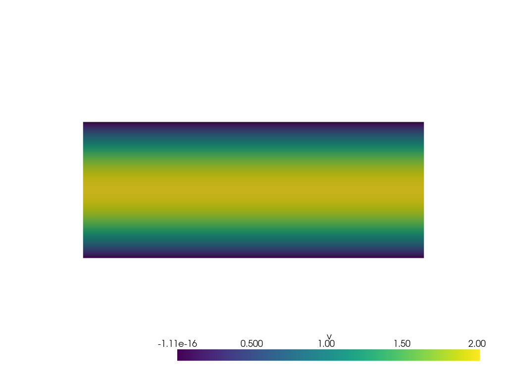
-component of the velocity field
Boundary Conditions and a Mass Source
Apart from the time integrator for the ADE, our simulation will still need boundary conditions at its walls. Also, for anything at all to happen, we would like to inject a fixed amount of the concentration into the medium at a certain point.
Define the Boundary Conditions
We would like to use two different kinds of boundary conditions in our simulation:
On the west, north, and south borders of , we apply a homogenous Dirichlet boundary condition; that is, we want to set at all times.
At the eastern border, we are going to place an outflow where the concentration can leave the domain. We model this using a Neumann boundary condition:
Interestingly, we can realize the Dirichlet boundaries simply by doing nothing at all.
The PatchData has initialized the arrays for c and c_next to zero;
and if you have correctly configured the iteration region of your time integrator,
the values at the boundary will stay at zero for all time.
Notebook Cell
@ps.flow.operator(target=target, ispace=Ω.vertices[-1, :])
def neumann_outflow(_eq):
    _eq.store[c()] = c[-1, 0]()
Inject a Mass Source
Last, to complete our simulation setup, we would like to inject some concentration into our system using a circular mass source.
We do so by fixing the concentration to within the circle with radius around the point
.
This leads us to a situation where we need to write an operator
that performs this operation only on an irregularily shaped (circular) part of the domain.
Restricting the operator’s iteration space to that circle using ispace is rather difficult,
so we instead use another way: we are going to construct a guarded operator.
Pystencils allows us to guard parts of an operator according to given conditions;
they will only be executed when these conditions evaluate to true.
In our case, our operator has two parts:
The equations to compute the distance of the current grid node to the circle’s center point ,
and the guarded portion that writes only if .
We realize these parts by splitting our operator into blocks, and by connecting these blocks accordingly.
We use the ps.flow.block and ps.flow.guarded_block decorators to create regular and guarded blocks, respectively.
Notebook Cell
@ps.flow.operator(target=target)
def constant_source():
    x, y, cx, cy, radius, d = sp.symbols("x, y, cx, cy, radius, d")

    @ps.flow.block
    def compute_distance(_eq):
        _eq.let[x, y] = Ω.vertex()
        _eq.let[cx, cy] = L[0] / 4, L[1] / 2
        _eq.export[radius] = L[1] / 10
        _eq.export[d] = sp.sqrt((x-cx)**2 + (y-cy)**2)

    @ps.flow.guarded_block(d < radius, preds=[compute_distance])
    def inject_source(_eq):
        _eq.store[c()] = 1

    return inject_source
Run the Simulation
Finally, all the ingredients are in place, and we can run our simulation. Let’s first define the full integration routine:
def integrate():
    neumann_outflow(Ω_data)
    constant_source(Ω_data)
    integrate_ade(Ω_data)
    Ω_data.swap(c, c_next)
The integration loop is built to run a given number nsteps of time steps,
and to extract snapshots of the field at a given frequency, in order to later
visualize the time series:
def simloop(nsteps, capture_freq=100):
    c_frames = []
    for t in range(nsteps):
        if t % capture_freq == 0:
            c_frames.append(Ω_data.asnumpy(c))
        integrate()

    return c_frames
Let’s run the simulation for 4000 time steps, and then visualize the result.
Ω_data[c][:] = 0.

c_frames = simloop(4000)
We again use PyVista to look at our simulation results. In the Jupyter notebook, you can use the following cell to create an interactive widget for exploring the captured time series:
pl = pv.Plotter()
mesh = Ω_data.viz().get_mesh()
pl.add_mesh(mesh, scalars="c", scalar_bar_args=dict(vertical=True, position_y=0.25),)
pl.set_position((0, 0, 3), reset=True)

if interactive_plots:
    #   Add a slider widget to seek through the time series
    def update_c(step):
        step = int(step)
        mesh.point_data["c"] = c_frames[step].flatten(order="F")

    pl.add_slider_widget(
        callback=update_c,
        rng=[0, len(c_frames)],
        value=0,
        title="time",
        interaction_event="always",
        style="modern",
        pointa=(0.1, 0.1),
        pointb=(0.7, 0.1),
    )

pl.show()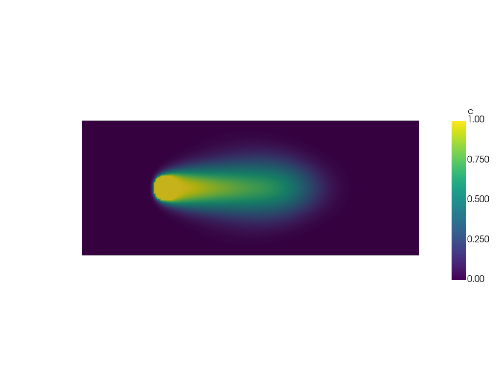
Concentration after time steps
If everything went well, you can see how a trail of advected material develops in the wake of the mass source. The larger the diffusivity , the wider the trail will grow. You can now experiment by running the simulation with different values for the diffusivity, but also different time intervals .
Conclusion
This concludes our lesson on implementing an explicit solver for the ADE in pystencils. We have seen how to configure operators to run on the GPU; how to bridge the patch data to PyVista for visualizaton, and how to use guarded kernels to apply operations only in certain regions of our domain. The end result is your first simulation of a time-dependent problem in pystencils; we will see many more of these in the following lessons.
If you have one.