The core of pystencils is an algebraic domain-specific language (DSL) designed to declaratively describe short-range array operations, so-called stencils. That language is based on a symbolic abstraction of discrete fields on numerical grids, which are used in writing numerical kernels as mathematical equations. Pystencils will then translate these to high-performing low-level code, which can be run on NumPy arrays. This lesson introduces the fundamental concepts of the pystencils DSL: domains modelled as patches, the fields defined on these, and finally stencil operators that evaluate equations and compute the values of these fields.
In the course of this lesson, you will
set up patches as the domain for your numerical fields;
declare fields to represent functions discretized on a patch’s grid;
write finite-difference stencil operators for numerically approximating derivatives on these fields;
investigate the low-level C++ code generated by pystencils for your operators;
measure the runtime of a 2D gradient operator, and evaluate its speed-up compared to a native NumPy implementation;
and, finally, parallelize the operator using OpenMP to make it even faster.
To begin, let’s import SymPy and pystencils.
import sympy as sp
import pystencils as ps
Numerical Domains: The Patch
The primary application area of pystencils is the numerical solving of partial differential equations (PDEs). Such equations deal with functions (so-called fields) from some contiguous region to a value set , as well as their derivatives (see Figure 1):
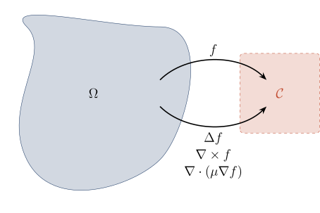
Figure 1:Function and some of its possible derivatives, as mappings from a region to their respective value sets.
To get started, we are first interested in the domain on which these functions are defined, for to solve a PDE numerically, we need to discretize using one or more appropriate grids. While (as in Figure 1) can be a region of arbitrary shape, to handle it numerically we need to impose some structure on it.
In pystencils, we employ a structured-grid approach to discretization, using regular cartesian grids. Our first assumption is that is a multi-interval spanned by its lower and upper corners (Figure 2):
![Multi-intervals \left[\boldsymbol{x^{\mathrm{min}}}, \boldsymbol{x^{\mathrm{max}}}\right] in one, two, and three dimensions.](/tutorial/build/MultiIntervals-1b035b4aa0840f2fc58a9c7dd1e65323.svg)
Figure 2:Multi-intervals in one, two, and three dimensions.
This -dimensional multi-interval is discretized using a cartesian grid of points:
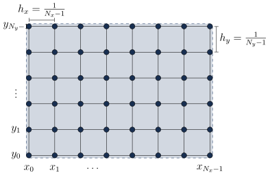
Figure 3:2D patch discretized using points. The discretization results in a grid with horizontal spacing and vertical spacing .
Such grid structures are represented in the language of pystencils by the class ps.grids.Patch.
Each patch gets a lower and an upper corner, as well as its number of vertices;
these parameters, as well as the patch itself, are symbolic (see lesson 1) mathematical objects.
Here’s how to create a patch ranging from to with vertices:
min_corner = sp.symbols("x_0, y_0")
max_corner = sp.symbols("x_1, y_1")

#   Use `dtype=ps.index_t` to indicate that N is an integer symbol
N = ps.symbols("N_x, N_y", dtype=ps.index_t)

Ω = ps.grids.Patch("Ω", min_corner, max_corner, num_vertices=N)
ΩDefining Fields on Patches
Now that we’ve established the discretization of the domain , let’s turn our attention to the codomain and define the fields themselves. In , pystencils primarily deals with tensors over the real numbers , giving rise to:
scalar fields:
vector-valued fields:
matrix-valued fields:
and fields holding higher-order tensors.
Tensor fields, as algebraic objects, are represented by the ps.grids.TensorField class.
We create a tensor field by giving it a name, underlying grid, and tensor shape:
u = ps.grids.TensorField("u", Ω.vertices, ())
uHere, we have created a scalar field (as denoted by the empty tensor shape ()), and placed it on the vertices of .
It is now a symbolic representation of a function from the set of grid points in to the real numbers .
Writing Stencil Operators
A stencil operator is a set of equations that compute new values for the entries of a field on each node , depending on ’s own entries, and the entries of other fields, only at the node and its direct neighborhood. Pystencils’ domain-specific language is designed to define such stencil operators as symbolic equations. In the following, we will get to know this language by looking at several simple, but common, stencil operators.
Common examples of stencil operators are finite-difference stencils that approximate a function’s derivatives using local difference quotients. Consider our scalar field
defined above. Its first spatial derivative in -direction can be approximated with a central-difference scheme:
Stencil Expressions
Using pystencils, we write the right-hand side of this finite difference stencil as a stencil expression:
h_x = sp.symbols("h_x")
dx_u = (u[1, 0]() - u[-1, 0]()) / (2 * h_x)
dx_uCompare the code in the above cell with the finite difference equation (2). They express the same thing, but with slightly different syntax. In particular, instead of writing the node coordinates as symbols, we access fields using stencil notation.
Assembling an Operator
On its own, the above is just an expression - but we want to go a step further, and evaluate that expression on actual numerical data. To do so, we create an operator. A pystencils operator is a set of stencil equations, like (2), that can be compiled to executable code and then evaluated on data stored in multidimensional arrays. Writing a pystencils operator is similar to writing a Python function, with a few differences. Here’s an example; an operator that computes the gradient of via central differences and stores the result in a vector field created for the purpose:
grad_u = ps.grids.TensorField("grad_u", Ω.vertices, (2,))

@ps.flow.operator(ispace=Ω.vertices[1:-1, 1:-1])
def compute_gradient(_eq):
    hx, hy = sp.symbols("h_x, h_y")
    _eq.let[hx] = Ω.spacing[0]
    _eq.let[hy] = Ω.spacing[1]

    _eq.store[grad_u(0)] = (u[1, 0]() - u[-1, 0]()) / (2 * hx)
    _eq.store[grad_u(1)] = (u[0, 1]() - u[0, -1]()) / (2 * hy)

compute_gradient
Output
Okay, that’s a lot of new syntax. Let’s take it apart:
The operator function is declared by decorating it with
@ps.flow.operator. Here, the operator’s iteration space is defined by slicing the vertex grid of . The expressionΩ.vertices[1:-1, 1:-1]removes the outermost slices of the grid from the iteration region, because at the borders the stencil expressions would involve field values from outside the grid, which do not exist.The function gets a single argument called
_eq. This object is used to collect the operator’s equations. Each equation has as its left-hand side either a symbol - making it a subexpression - or a field access, making it an update-expression. Subexpressions are declared using_eq.let, by assigning a right-hand side expression to a symbol. Similarly, field updates are written using_eq.store, signifying that the result of the given expression should be written to the field.
The result of defining compute_gradient is not a Python function, but an algebraic object; a collection of symbolic equations.
Pystencils will automatically convert this operator object to executable code.
We can even take a look under the hood, and see the code it generates, using ps.inspect:
ps.inspect(compute_gradient)Output
As you can see, pystencils turns the operator into a 2D loop nest. It will also perform a number of optimizations, such as precomputing constant values and drawing loop-invariant code outside of the loop nest.
Notebook Cell
@ps.flow.operator
def initialize_u(_eq):
    x, y = sp.symbols("x, y")
    _eq.let[x], _eq.let[y] = Ω.vertex()

    _eq.store[u()] = sp.sinh(2 * x) + sp.cos(4 * sp.pi * y)

initialize_uFrom Algebra to Numerical Computation
Now that we have some operators, it is time to apply them to actual numerical data. So far, everything we have constructed with pystencils has been algebraic; all equations and no data. This was the symbolic language layer of pystencils. That layer is complemented by the numerical runtime system offered by pystencils, which we will take a look at next.
The first step toward numerical evaluation is to set up the data behind our fields and symbols.
Every field needs an underlying data array,
and every symbol a numerical value.
To handle these, we use the ps.grids.PatchData data manager.
To create the patch data manager, we pass it our patch; a dictionary with values for any free symbols we have used in our
definitions so far; as well as a list of fields for which arrays should be created:
Ω_data = ps.grids.PatchData(
    Ω,  # the patch
    {
        # dictionary that sets numerical values for any free symbols
        # i.e. parameters of Ω
        min_corner: (0, 0),
        max_corner: (1, 1),
        N: (32, 32)
    },
    fields=[u, grad_u]  # list of fields for which data arrays should be allocated
)
Let’s examine what we created here. Using Ω_data[x], you can access and view the data behind the symbol, or field, x.
For instance, we can see that u is now backed by a NumPy array of shape (32, 32), which is exactly the number of vertices on the patch:
Ω_data[u]array([[0., 0., 0., ..., 0., 0., 0.],
[0., 0., 0., ..., 0., 0., 0.],
[0., 0., 0., ..., 0., 0., 0.],
...,
[0., 0., 0., ..., 0., 0., 0.],
[0., 0., 0., ..., 0., 0., 0.],
[0., 0., 0., ..., 0., 0., 0.]], shape=(32, 32))To run an operator on the data managed by Ω_data, simply call it with the data manager as its only argument.
For instance, let’s run initialize_u and take a look at the resulting state of u.
initialize_u(Ω_data)Notebook Cell
%matplotlib agg

import matplotlib.pyplot as plt
import numpy as np

def plot_surface(field):
    xs = np.linspace(Ω_data[min_corner[0]], Ω_data[max_corner[0]], Ω_data[N[0]])
    ys = np.linspace(Ω_data[min_corner[1]], Ω_data[max_corner[1]], Ω_data[N[1]])
    xx, yy = np.meshgrid(xs, ys, indexing="ij")
    field_data = Ω_data[field]

    fig, ax = plt.subplots(subplot_kw=dict(projection="3d"))
    ax.plot_surface(xx, yy, field_data)
    return fig
plot_surface(u)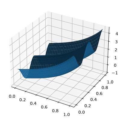
Notebook Cell
compute_gradient(Ω_data)Notebook Cell
def plot_quiver(field):
    xs = np.linspace(Ω_data[min_corner[0]], Ω_data[max_corner[0]], Ω_data[N[0]])
    ys = np.linspace(Ω_data[min_corner[1]], Ω_data[max_corner[1]], Ω_data[N[1]])
    xx, yy = np.meshgrid(xs, ys, indexing="ij")
    field_data = Ω_data[field]

    fig, ax = plt.subplots()
    ax.quiver(xx, yy, field_data[:,:,0], field_data[:,:,1])
    return fig
plot_quiver(grad_u)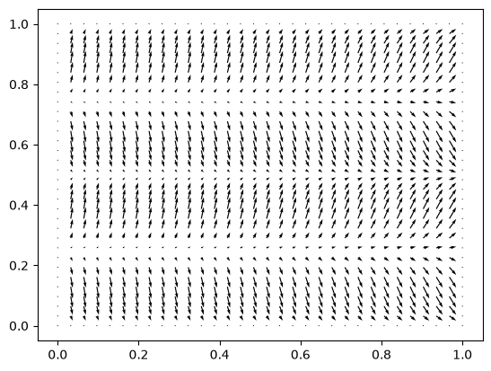
If everything went right, you should see a vector field pointing from the troughs to the peaks of the cosine wave in -direction, with a slight tilt upward in -direction.
Performance Comparison and Optimization
Through its just-in-time compilation system, with its abilities to hardware-accelerate and optimize numerical operators on the fly, pystencils is able to outperform native Python, as well as purely NumPy-based, numerical code by a significant margin. Even without optimizations enabled, we can expect our gradient operator to run significantly faster than an equivalent NumPy-based implementation.
pystencils vs NumPy
Let’s see how much speed-up we can actually get in practice. The following cell contains a pure NumPy-implementation of the gradient operator:
def gradient_numpy(u, grad_u):
    Nx, Ny = u.shape
    hx = 1. / (Nx - 1)
    hy = 1. / (Ny - 1)

    grad_u[1:-1,1:-1,0] = (u[2:,1:-1] - u[0:-2,1:-1]) / (2 * hx)
    grad_u[1:-1,1:-1,1] = (u[1:-1,2:] - u[1:-1,0:-2]) / (2 * hy)
We’re now going to benchmark gradient_numpy against our compute_gradient operator.
For a reliable measurement, however, we’ll need data structures that are much larger than what we experimented with above.
Notebook Cell
benchmark_data = ps.grids.PatchData(
    Ω,
    {
        min_corner: (0, 0),
        max_corner: (1, 1),
        N: (1000, 1000)
    },
    fields=[u, grad_u]  # list of fields for which data arrays should be allocated
)
%%timeit
compute_gradient(benchmark_data)1.1 ms ± 157 μs per loop (mean ± std. dev. of 7 runs, 1,000 loops each)
Notebook Cell
%%timeit
gradient_numpy(benchmark_data[u], benchmark_data[grad_u])4.71 ms ± 90 μs per loop (mean ± std. dev. of 7 runs, 100 loops each)
Depending on your hardware, you should be able to see the pystencils operator run several times faster than the NumPy equivalent.
Optimization: Thread-Parallel Execution using OpenMP
Let’s take this one step further. One major advantage of pystencils is that it allows us to apply various optimizations to the generated operator code.
For instance, we can choose to use OpenMP to run our kernel with multiple threads in parallel,
to share the work among several CPU cores.
Let’s try that for compute_gradient, and see if we can get an even larger speed-up.
To enable OpenMP, we will first have to clear the generated code of our operator:
compute_gradient.clear()We can now reconfigure the code generator through the operator’s .config property.
We enable OpenMP, using static scheduling and four threads:
compute_gradient.config.cpu.openmp.enable = True
compute_gradient.config.cpu.openmp.schedule = "static"
compute_gradient.config.cpu.openmp.num_threads = 4Now, let’s regenerate the operator’s code, and see if, and where, the OpenMP directives were added (note: calling ps.inspect automatically causes the code to be generated):
ps.inspect(compute_gradient)Output
As you should be able to see, a #pragma omp parallel with the given number of threads was added outside of the loop nest, followed by a #pragma omp for work-sharing construct.
Notebook Cell
compute_gradient.compile_code()Notebook Cell
%%timeit
compute_gradient(benchmark_data)553 μs ± 3.66 μs per loop (mean ± std. dev. of 7 runs, 1,000 loops each)
Conclusion
In this lesson, we have gotten to know some of the fundamental components of the pystencils kernel language: patches, fields, stencil notation, and operators. We have seen how to apply these in computing finite differences, and have observed how pystencils operators can achieve significant speed-up over purely NumPy-based code.
With these fundamentals in our pack, we can move on to apply pystencils to actual numerical problems. In the next lessons, we will use pystencils to numerically solve the Poisson and Advection-Diffusion equations; in doing so, we will further explore the features of pystencils’ DSL, and try out its capabilities for high-performance code generation, e.g. through GPU acceleration.