Poisson’s Equation is one of the most fundamental elliptic partial differential equations (PDEs) out there. Given a region , and scalar fields , the Poisson equation reads
where is the Laplace operator, signifying the divergence of the gradient of . Solving the Poisson equation numerically qualifies as the classic ‘Hello World’ example of numerics. Hence, it should come as no surprise that in this lesson, we will construct a simple solver for the traditional five-point finite difference discretization of (1).
By the end of this lesson, you will have implemented a solver for a boundary value problem of Poisson’s equation in 2D. On the way, you will
Use the
Patchclass to define a numerical domain, set up fields on its vertex grid, and work with its geometry;Manage simulation data for a patch using
PatchData;Symbolically derive a Jacobi-style update kernel from a finite difference equation and implement it as a pystencils operator;
and use reductions to evaluate a global error measure for your solver.
Let’s start by importing the packages we will need.
import sympy as sp
import pystencils as ps
import numpy as np

import matplotlib.pyplot as plt
Model Problem
We will consider the following model problem for the Poisson equation on the unit square :
with the known source function
and the Dirichlet boundary condition
The problem definition is illustrated in Fig. 1.
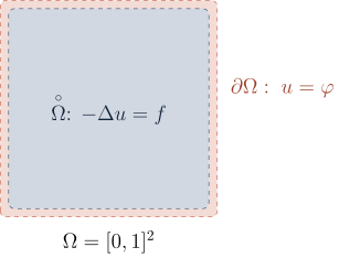
Figure 1:The model problem for the Poisson-Equation.
In this lesson, we will develop a numerical solver for a finite-difference discretization of this problem, based on the Jacobi method. For this, we discretize with a regular cartesian grid of points, which gives rise to a grid spacing of (see Fig. 2):
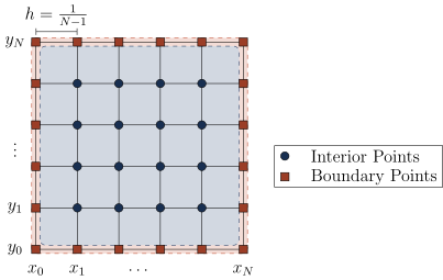
Figure 2:Numerical grid for our solver. The functions and are represented by their values on the grid points, and the boundary value problem (2) is discretized by a system of linear equations, one for each grid point.
Set up Algebraic Objects
We start off by creating symbols and the patch object for our simulation grid.
Notebook Cell
N = ps.symbols("N", dtype=ps.index_t)
Ω = ps.grids.Patch("Ω", (1, 1), num_vertices=(N, N))
ΩNotebook Cell
u = ps.grids.TensorField("u", Ω.vertices, ())
f = ps.grids.TensorField("f", Ω.vertices, ())

uInitialize the Fields
Next, we need to set up the fields and to reflect the boundary-value problem (2).
The entries of f must be set to the corresponding values of ,
while u must be set to only on the boundary points.
Notebook Cell
@ps.flow.operator
def initialize_model_problem(_eq):
    x, y = sp.symbols("x, y")
    _eq.let[x, y] = Ω.vertex()
    _eq.store[f()] = sp.pi**2 * ( 4 * sp.sin(2 * sp.pi * x) + 16 * sp.cos(4 * sp.pi * y) )

    _eq.store[u()] = sp.Piecewise(
        (
            sp.sin(2 * sp.pi * x) + sp.cos(4 * sp.pi * y),
            sp.Or(sp.Eq(x, 0), sp.Eq(x, 1), sp.Eq(y, 0), sp.Eq(y, 1)),
        ),
        (0, True)
    )
To run our solver for an actual incarnation of the problem (2), we need to create data structures (i.e. arrays) for the patch and its fields.
Notebook Cell
Ω_data = ps.grids.PatchData(Ω, {N: 32}, fields=[u, f])We can now run our initialization operator on the data arrays:
initialize_model_problem(Ω_data)Let’s look at our initial state. We will use the following function to visualize the scalar fields as surface plots:
Notebook Cell
def plot_surfaces(arrs: dict[str, np.ndarray], **kwargs):
    fig, axes = plt.subplots(1, len(arrs), subplot_kw=dict(projection="3d"), **kwargs)
    if len(arrs) == 1:
        axes = [axes]

    for ax, (title, arr) in zip(axes, arrs.items()):
        N, _ = arr.shape
        cs = np.linspace(0, 1, N)
        xx, yy = np.meshgrid(cs, cs)

        ax.set_title(title)
        ax.set_xlabel("x")
        ax.set_ylabel("y")

        ax.plot_surface(xx, yy, arr)
When visualizing, we should see that f shows a superposition of two waves as defined in (3),
and that u is set to a similar superposition only at the edges:
plot_surfaces({"u": Ω_data[u], "f": Ω_data[f]}, figsize=(12, 8))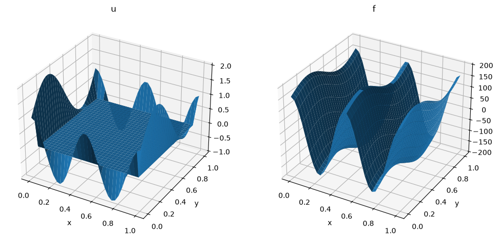
That’s the initial state done. Let’s continue by discretizing the Poisson equation (1) and setting up the Jacobi smoother.
The Jacobi Smoother
Discretizing the Laplace Operator on the grid using second-order finite differences yields the following discrete stencil operator :
The discretized boundary-value problem therefore reads
This is a system of linear equations, which we are going to solve iteratively using the Jacobi method.
Notebook Cell
u_tmp = ps.grids.TensorField("u_tmp", Ω.vertices, ())

@ps.flow.operator(ispace=Ω.vertices[1:-1, 1:-1])
def jacobi_step(_eq):
    h = sp.Symbol("h")
    _eq.let[h] = Ω.spacing[0]

    poisson_equation = ( 4 * u[0,0]() - u[-1, 0]() - u[1, 0]() - u[0, 1]() - u[0, -1]() ) / h**2 - f()
    jacobi_rule = sp.solve(poisson_equation, u())[0]

    _eq.store[u_tmp()] = jacobi_rule
To run the smoother, we first need to create an array for the new field u_tmp.
To honor the boundary conditions, we initialize it as a copy of u:
Ω_data.add_field(u_tmp, copy_of=u)Let’s now run the Jacobi smoother, say, for 200 iterations.
After each step, we must swap the data arrays of u and u_tmp:
for _ in range(200):
    jacobi_step(Ω_data)
    Ω_data.swap(u, u_tmp)
After 200 steps, we should see that u has taken a form similar to f, as a superposition of two waves:
plot_surfaces({"u": Ω_data[u]})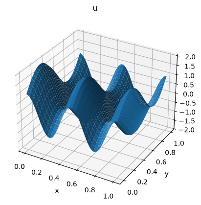
Error Evaluation
As a last step in this lesson, would like to numerically evaluate the accuracy of the approximate solution u
by computing the -Norm of the error.
To do so, we observe that the model problem (2) is solved exactly by the analytical solution
which, unsurprisingly, is identical to the boundary function . We would like to compute the error vector , and evaluate its supremum norm
For this, we set up a new field e for the error vector, and a typed symbol e_norm for computing the norm:
e = ps.grids.TensorField("e", Ω.vertices, ())
e_norm = ps.symbols("e_norm", dtype=ps.numeric_t)Notebook Cell
@ps.flow.operator
def compute_error(_eq):
    h, u_ana, x, y = sp.symbols("h, u_ana, x, y")

    _eq.let[x, y] = Ω.vertex()
    _eq.let[h] = Ω.spacing[0]

    _eq.let[u_ana] = sp.sin(2 * sp.pi * x) + sp.cos(4 * sp.pi * y)

    _eq.store[e()] = u() - u_ana
    _eq.reduce[e_norm, "max"] = sp.Abs(e())
Let’s add an array for the error vector to our patch data:
Ω_data.add_field(e)Let’s plot the progression of the error during the 200 iterations of our solver loop. For this, we set up an array with room for 200 values of ":
e_norms = np.zeros((200,))Next, we reset our arrays by running initialize_model_problem again.
In the loop, we call compute_error after each iteration, pointing e_norm at the entry t of our prepared array.
Note that we need to use the slice syntax [t:t+1] such that NumPy gives us a view into the array, instead of just copying out the value:
initialize_model_problem(Ω_data)

for t in range(200):
    jacobi_step(Ω_data)
    Ω_data.swap(u, u_tmp)
    compute_error(Ω_data, e_norm=e_norms[t:t+1])
With the following cell, we plot the error progression. It should follow a roughly inverse-exponential curve, as the error is reduced multiplicatively by a roughly constant factor at each step.
fig, ax = plt.subplots()
ax.grid()
ax.set_xlabel(r"$t$")
ax.set_ylabel(r"$\Vert \boldsymbol{e} \Vert_{\infty}$")
ax.plot(range(200), e_norms)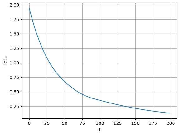
Conclusion
Congratulations! You have constructed your first numerical solver using pystencils, with many common ingredients: The initial setup, an iterative solution routine, and an error evaluation and validation step.
In the next lesson, we’ll apply the same techniques, and more, to solve a time-dependent advection-diffusion problem.