The Lattice Boltzmann Method (LBM) is a methodological approach to the simulation of transport phenomena that differs from classical “finite-X” [1] methods in that it doesn’t solve the relevant PDEs directly; but does so through a statistical, mesoscopic approach. Its predominant application is the simulation of fluids following the Navier-Stokes Equations, for which it is derived from the Boltzmann equation.
If you are not yet familiar with the fundamentals of the LBM, we recommend that you take on these lessons in combination with studying LBM theory, using textbooks such as Krüger et al. (2017).
For computational fluid dynamics (CFD), the LBM is attractive due to its relative algorithmic simplicity. Due to the locality of its operations it is straightforwardly parallelizable and performs well on modern supercomputing hardware.
The term LBM nowadays covers a huge ecosystem of different models based on the common LBM discretization scheme. The Python package lbmpy, which we will get to know in this lesson, implements a significant subset of these in purely symbolic algebra, based on pystencils.
This lesson explores the basic functionalities of lbmpy by applying it to a popular benchmark problem of CFD: the Taylor-Green Vortex (TGV) Decay scenario.
By the end of this lesson, you will have created, run, and evaluated a numerical solver for the TGV decay scenario using pystencils and lbmpy. On the way, you will
define the basic algebraic ingredients of a simple D2Q9 BGK lattice Boltzmann method using lbmpy;
configure and derive the essential operations of the LBM, namely initialization, collision, streaming, and export of observables;
set up a fully periodic simulation domain and implement periodic streaming;
evaluate your simulation method’s correctness and accuracy with respect to an analytical solution.
Let’s start by importing what packages we need. When working in a Jupyter notebook, use the cells below to activate interactive plotting with PyVista.
import sympy as sp
import pystencils as ps
import numpy as np
import matplotlib.pyplot as plt
import pyvista as pv

interactive_plots = FalseSimulation Domain
The Taylor-Green Vortex Decay scenario we consider in this lesson lives on a fully periodic square domain with sidelengths ; i.e. our simulation space will be . This space will be discretized uniformly using cells, on which we will later run our lattice Boltzmann solver.
Notebook Cell
N = ps.symbols("N", ps.index_t)
Ω = ps.grids.Patch("Ω", (2 * sp.pi,) * 2, num_cells=(N, N))
Initial State and Analytical Solution
The density and velocity fields of the two-dimensional Taylor-Green vortex is described by the following time-dependent equations:
The flow field depends on two free parameters:
The fluid’s kinematic viscosity ;
the characteristic (maximum) velocity .
Notebook Cell
u_0, ν, t = ps.symbols("u_0, nu, t")
rho = ps.grids.TensorField("rho", Ω.cells, ())
u = ps.grids.TensorField("u", Ω.cells, (2,))

@ps.flow.operator
def tgv_analytical(_eq):
    x, y = sp.symbols("x, y")
    _eq.let[x, y] = Ω.cell_center()

    rho_decay, u_decay = sp.symbols("rho_decay, u_decay")

    _eq.let[rho_decay] = sp.Rational(3, 4) * u_0**2 * sp.exp(-4 * ν * t)
    _eq.store[rho()] = 1 - rho_decay * (sp.cos(2 * x) + sp.cos(2 * y))

    _eq.let[u_decay] = u_0 * sp.exp(-2 * ν * t)
    _eq.store[u(0)] = u_decay * sp.sin(x) * sp.cos(y)
_eq.store[u(1)] = - u_decay * sp.cos(x) * sp.sin(y)Notebook Cell
Ω_data = ps.grids.PatchData(
    Ω,
    {
        N: 256,
        ν: 1. / 6.,
        u_0: 0.25
    },
    fields=[rho, u]
)
Notebook Cell
tgv_analytical(Ω_data, t=0)You can use the function plot_u_streamlines in the following cell to visualize the velocity field’s streamlines.
If you did everything correctly, you should see a square of four counter-rotating vortices; the fluid remaining stationary at their centers, and moving with a maximum speed of at their contact points.
Notebook Cell
def plot_u_streamlines():
    import pyvista as pv
    mesh = Ω_data.viz(fix_vectors=[u]).get_mesh()

    pmesh = mesh.cell_data_to_point_data()
    streamlines1 = pmesh.streamlines(
        u.name,
        n_points = 25,
        pointa=(0.5 * np.pi, 0, 0),
        pointb=(0.5 * np.pi, 2. * np.pi, 0)
    )
    streamlines2 = pmesh.streamlines(
        u.name,
        n_points = 25,
        pointa=(1.5 * np.pi, 0, 0),
        pointb=(1.5 * np.pi, 2. * np.pi, 0)
    )

    pl = pv.Plotter()
    pl.add_mesh(streamlines1.tube(radius=0.01))
    pl.add_mesh(streamlines2.tube(radius=0.01))
pl.show()plot_u_streamlines()2026-09-30 07:07:55.588 ( 4.058s) [ 79A3255E0200]vtkXOpenGLRenderWindow.:1452 WARN| bad X server connection. DISPLAY=
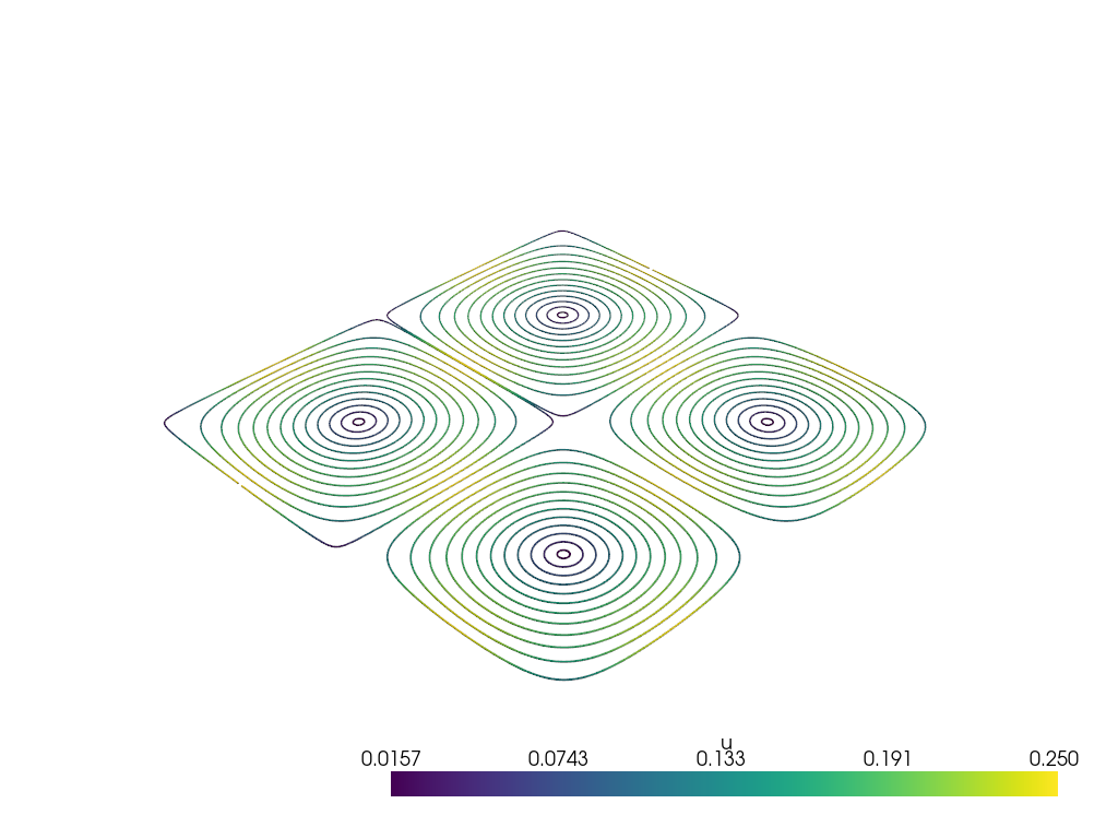
Figure 1:Velocity streamlines of the initial state.
The Lattice Boltzmann Solver
Our goal for this lesson is to simulate the time evolution of the TGV flow state with the lattice Boltzmann method. We will use lbmpy to construct the four central operations of our solver:
Initialization of the LBM’s particle distribution functions from the initial density and velocity fields;
Collision of particle distributions at each cell;
Streaming of the particles from each cell to its neighbors; and
Export of the updated values for density and velocity for evaluation and post-processing.
For each, lbmpy provides pre-defined operators which we merely have to configure with the details of our chosen lattice Boltzmann method. Before we get to them, we first have to define our discretization scheme by selecting a stencil and lattice structure. We then continue with the collision operator, as the derivations of the other operators depend on it.
Spatial Discretization: Stencil and Lattice
A wide range of different collision models has been developed under the umbrella of “lattice Boltzmann methods”, and many of these are implemented within lbmpy; from the most basic BGK scheme to advanced cumulant-based collision operators. For the purposes of this lesson, we will start small, using the classical single-relaxation time BGK method on a D2Q9 lattice.
The D2Q9 velocity set discretizes the density distribution function of the Boltzmann equation using nine velocities in two dimensions:
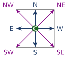
Figure 2:The D2Q9 velocity set. The stationary velocity is marked in green; the primary velocities in blue, and the secondary velocities in purple. Directions are abbreviated according to compass directions (North, South, East, West) and Center.
In lbmpy, velocity sets are represented by the LBStencil class. Let’s create an LBStencil instance for D2Q9:
from lbmpy import LBStencil

d2q9 = LBStencil("D2Q9")
d2q9When printing the stencil in a Jupyter notebook, you get an overview of its velocities and their numbering.
According to the D2Q9 velocity set, in the LBM we store and manipulate a local distribution vector on each cell of our grid . There, the entry represents the relative number of particles at moving with the velocity . Assembling all these local distributions into a field , we get the underlying lattice for our simulation:
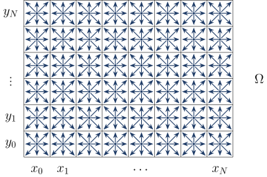
Figure 3:A 2D lattice using the D2Q9 velocity set. Each cell holds an ensemble of nine discrete populations.
The lattice we represent using the Lattice class from the lbmpy.lattice module.
The following cell creates a lattice, and immediately adds it to Ω_data to prepare its data array:
from lbmpy import lattice

f = lattice.Lattice("f", d2q9, Ω.cells)
Ω_data.add_field(f)
fThe Collision Operator
The classical BGK collision operator, which we will use for our simulation, is given by eq. 3:
where is the equilibrium distribution, and designates the relaxation rate. For the equilibrium distribution, we are using the second-order Hermite expansion of the isothermal Maxwell-Boltzmann equilibrum (eq. 4):
with the lattice weights, and the lattice speed of sound. The local density and velocity are computed as moments of the pre-collision population vector :
The relaxation rate is directly related to the kinematic viscosity as
We could now go about implementing these equations manually as a pystencils operator. Luckily, lbmpy saves us that effort as these collision equations, and many more, are already realized via its algebraic derivation engine.
To define lattice Boltzmann collision schemes in lbmpy, we need to construct an object of the LBMConfig class.
To its constructor we pass the various settings and ingredients of our methods:
the velocity set (
stencil=d2q9);the collision method (
method=Method.SRT);the relaxation rate (
relaxation_rate=...)and settings controlling the equilibrium distribution (i.e.
compressible=Trueto get the weakly compressible form of the LBM).
Once our configuration is complete, we tell lbmpy to derive the collision equations as a pystencils flowgraph by creating an object of the class
lattice.Collide.
Hint
You can use lbmpy.relaxation_rate_from_lattice_viscosity to convert to .
from lbmpy import Method, LBMConfigNotebook Cell
from lbmpy import relaxation_rate_from_lattice_viscosity

lbm_config = LBMConfig(
    stencil=d2q9,
    method=Method.SRT,
    relaxation_rate=relaxation_rate_from_lattice_viscosity(ν),
    compressible=True
)

collide = lattice.Collide(f, lbm_config)
collideNotebook Cell
collide_op = ps.flow.Operator(collide)Solution to Exercise 4
There’s a few differences between the BGK equations given in this text, and the equations derived by lbmpy:
lbmpy splits up the computation of and as well as the equilbirium to reduce the number of arithmetic operations to a minimum
Furthermore, notice that lbmpy introduces a quantity , and sets . This realizes the numerical optimization known as zero-centering, which improves the algorithm’s numerical stability especially for
float32-based implementations. For details, see Hennig et al. (2023).
The Streaming Step
The collision operation is one of two operations that make up the explicit lattice Boltzmann time-stepping scheme. The second is the streaming step, where all post-collision populations move to their neighboring cells according to their lattice velocities:
In lbmpy, the streaming step (7) is executed by the lattice.Advance operation.
Notebook Cell
advance_f = lattice.Advance(f)Lattice Initialization and Export of Observables
Before we can begin the LBM time integration, the lattice f needs to be initialized to reflect the initial state given by (1).
We will use an initialization to equilibrium, where all populations are set to
the equilibrium values (see (4)).
This is realized by the SetEquilibrium graph, which is defined in the lbmpy.lattice module.
The following cell creates a pytencils operator from an instance of SetEquilibrium.
The SetEquilibrium graph takes four arguments:
The lattice
f, to which the equilibrium state will be written;The lattice Boltzmann method object contained in your
Collidegraph, which defines relevant information needed to derive the initialization equations (the equilibrium distibution, etc);and finally the fields
rhoanduwhich provide the initial fluid density and velocity.
Run the following cell to create and print the initialization graph.
set_eq = ps.flow.Operator(
    lattice.SetEquilibrium(f, collide.method, rho, u)
)
set_eq
Output
SetEquilibrium is used to initialize the LBM’s populations from an initial state, turning density and velocity values to associated distribution functions.
However, to evaluate the results of our simulation, we also need to go in the other direction:
extract the momentary density and velocity values from the LBM’s distributions,
and write them out to the fields rho and u.
This is done by the ExportMacroscopics flowgraph from the lattice module.
Notebook Cell
export_macros = ps.flow.Operator(
    lattice.ExportMacroscopics(f, collide, rho, u)
)

export_macrosPeriodic Streaming
As mentioned in the beginning of this lesson, the Taylor-Green vortex scenario is fully periodic. For the LBM, this means that during the streaming step, populations moving across the edges of must re-enter the domain on its opposite side, as illustrated in figure 4:
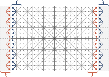
Figure 4:Periodic streaming in -direction. Populations leaving the domain on the western edge must re-enter in the east, and populations leaving at the eastern border come back in at the western border. In the TGV scenario, the same needs to happen in -direction.
Periodic streaming is realized by the lbmpy operator lattice.PeriodicStream.
Notebook Cell
periodic_stream = lattice.PeriodicStream(f, (True, True))LBM Integration Loop
Finally, all ingredients are in place to create our lattice Boltzmann solver loop. Here’s a few basic rules for implementing an LBM time stepping scheme in lbmpy:
SetEquilibriuminitializes a lattice to a fully defined pre-collision state. This means that the first operation of the LBM solver must be a collision, followed immediately by streaming.All other operations (we can call them support operations) share a common task: to reconstruct any missing input populations to the next collision step. In our case, only the periodic stream operator falls into this category, as it provides the missing distribution values at the domain edges.
ExportMacroscopicsis designed to extract the simulation’s observables from a pre-collision state. It must therefore come after all support operations, but before collision.
Notebook Cell
def lbm_step(with_export: bool = False):
    if with_export:
        export_macros(Ω_data)

    collide_op(Ω_data)
    advance_f(Ω_data)
    periodic_stream(Ω_data)
Evaluation: Kinetic Energy
When running the simulation, we’d like a quantitative assessment of its results and their accuracy. Here, the TGV scenario comes in very handy, as it is one of very few known analytical solutions to the Navier-Stokes equations. We know its desired behavior exactly (eq. 1) and can thus use it to evaluate the correctness of our numerical method.
Instead of checking against the solution directly, in this lesson we will instead evaluate the total kinetic energy in the TGV system. As the vortices slow down each other due to viscous friction, the system’s momentum, and therefore kinetic energy, decay exponentially over time.
The total kinetic energy of the discrete TGV system is given as
where is the volume of the cell . We will later compare this to the analytical solution for , which by integration is found to be
Notebook Cell
E_kin = ps.symbols("E_kin", dtype=ps.numeric_t)

@ps.flow.operator
def compute_ekin(_eq):
    V = sp.symbols("V")
    _eq.let[V] = Ω.spacing[0] * Ω.spacing[1]
    _eq.reduce[E_kin, "+"] = V * rho() / 2 * (u(0)**2 + u(1)**2)
Run the Simulation
Now all that’s left is to run the simulation and evaluate its results.
Notebook Cell
def tgv_loop(n_steps: int, n_out: int | None = None):
    if n_out is None:
        n_out = n_steps // 10

    ekin_size = n_steps // n_out
    ekin_values = np.zeros(ekin_size, dtype=Ω_data.default_dtype)

    for i in range(n_steps):
        do_export = ((i % n_out) == 0)

        lbm_step(do_export)

        if do_export:
            sample_idx = i // n_out
            compute_ekin(Ω_data, E_kin=ekin_values[sample_idx:sample_idx+1])

    return ekin_values
Now it is finally time to initialize all data structures and run the simulation.
Notebook Cell
n_steps = 5000
n_out = 500

#  Reset simulation data
tgv_analytical(Ω_data, t=0)
set_eq(Ω_data)

#  Run n_steps
ekin_values = tgv_loop(n_steps, n_out)

#  Plot streamlines
plot_u_streamlines()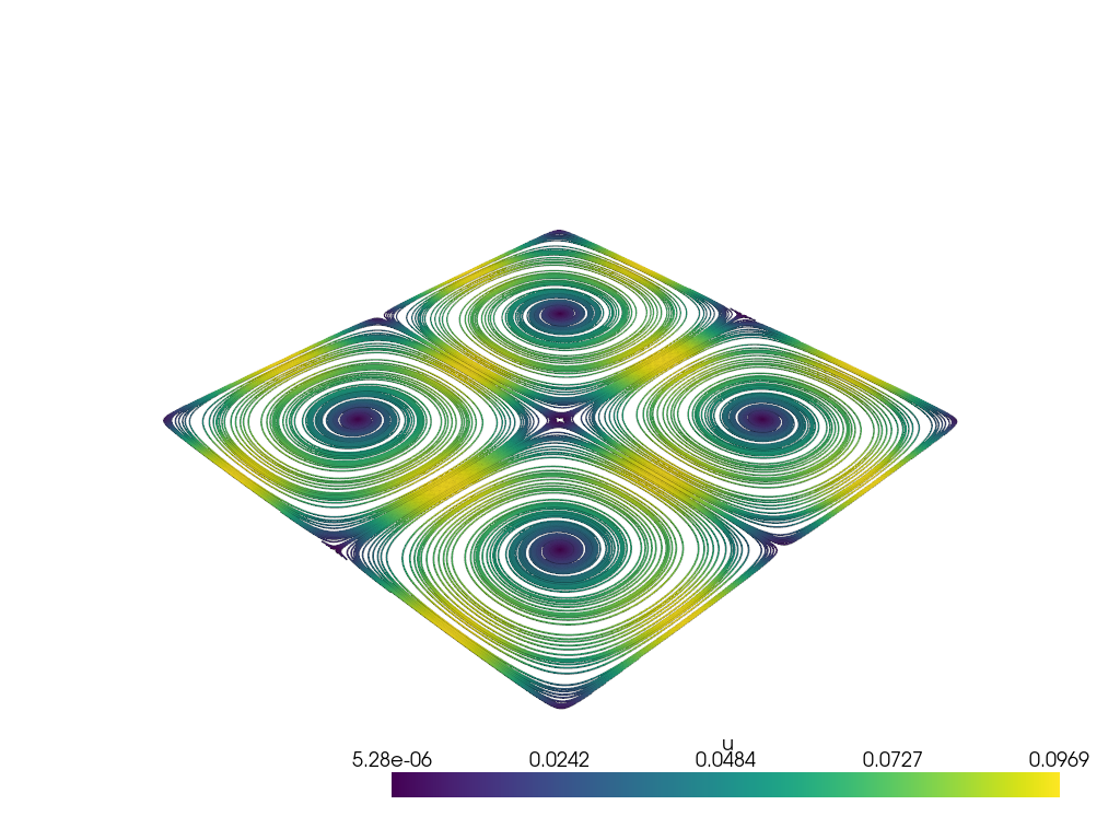
Notebook Cell
%matplotlib agg

def plot_ekin(ekin_values, n_out):
    fig, ax = plt.subplots()

    ax.grid(which="both")

    ax.set_xlabel("time steps")

    ax.set_yscale("log")
    ax.set_ylabel(r"$E^{\mathrm{kin}}$")

    ts = np.arange(0, len(ekin_values) * n_out, n_out)

    ax.plot(ts, ekin_values, label="Simulation", marker="s")

    ekin_analytical = Ω_data[u_0]**2 * np.pi**2 * np.exp(- 4 * Ω_data[ν] * (2. * np.pi / Ω_data[N])**2 * ts)
    ax.plot(ts, ekin_analytical, label="Analytical", color="black")

    ax.legend()

    return fig
plot_ekin(ekin_values, n_out)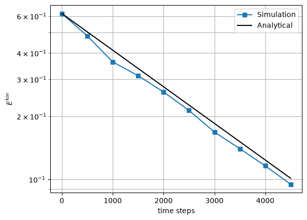
Figure 5:Progression of the kinetic energy, compared to the analytical solution.
If everything was done correctly, you should see the same streamlines profile as in the beginning - just with a uniformly lower velocity. Plotting the kinetic energy, you will see that the values from your simulation soon depart slightly from the analytical solution, but follow the same trend of exponential decay.
Conclusion
In this lesson, you have established first contact with the lbmpy library for lattice Boltzmann fluid simulations.
You have set up the fundamental algebraic objects of the LBM (namely the stencil and lattice);
and have configured the basic operations SetEquilibrium, Collide, Advance, ExportMacroscopics and PeriodicStream for the traditional BGK LBM scheme.
These you used to prepare and simulate the Taylor-Green Vortex Decay flow scenario,
for which you finally evaluated the progression of kinetic energy to evaluate your method’s correctness.
Congratulations!
Finite Differences, Finite Volumes, Finite Elements
- Krüger, T., Kusumaatmaja, H., Kuzmin, A., Shardt, O., Silva, G., & Viggen, E. M. (2017). The Lattice Boltzmann Method: Principles and Practice. In Graduate Texts in Physics. Springer International Publishing. 10.1007/978-3-319-44649-3
- Hennig, F., Holzer, M., & Rüde, U. (2023). Advanced Automatic Code Generation for Multiple Relaxation-Time Lattice Boltzmann Methods. SIAM Journal on Scientific Computing, 45(4), C233–C254. 10.1137/22m1531348
- Geier, M., & Schönherr, M. (2017). Esoteric Twist: An Efficient in-Place Streaming Algorithmus for the Lattice Boltzmann Method on Massively Parallel Hardware. Computation, 5(2), 19. 10.3390/computation5020019